You made it to the Neural Network series finale! It’s been a fascinating journey, but there’s still work to be done and questions to answer. So saddle up, grab a drink, and let’s jump right in. The Jupyter notebooks mentioned throughout can be found here.

Experiment 1-1: Less Filters

It’s often the case that clients want their networks deployed on mobile devices and ask to keep the networks as small as possible. So, potentially cutting down on the number of filters could be a huge win. Inspecting experiments/experiment1/ex1-1 will reveal several prepared notebooks. In ex1-1-train.ipynb, the number of filters per convolution layer was reduced by half. This yields a network with half the amount of parameters than the original model. 

The results on the testing set derived from CMU faces look great, 100%. Looking at ex1-1-test.ipynb, it looks like the tests on Gilbert, Ryan, Sarah, (the three amigos from Part 2) are also about the same. So, on one hand there’s a network that performs as well on the CMU faces data as our original network from experiment0. On the other hand, it performs as poorly as the experment0 network on the three amigos. Now, let us look at the visualization results. The entire set of visualizations can be seen in view_layers.ipynb. 

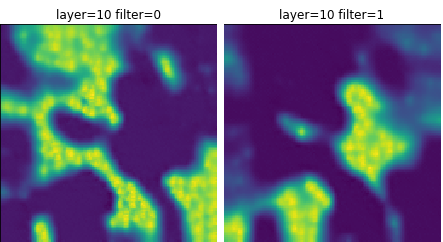
Image 1a: These HappyMaps for the experiment 1-1 decision layer look very familiar.

The first thing to notice is that the HappyMaps for dense_3, the decision layer, look about the same as they do for experiment0’s HappyMaps. This is a confirmation that the decisions made by the two networks are about the same. Before feature visualization, we would have to check the results on individual examples to see how they corresponded. With feature visualization, it’s clear from the get-go that yes, the decisions are about the same. So now there’s a network that is about half as big as the original AND has learned roughly the same thing. What’s more, there’s plenty of evidence to attest to that fact. 

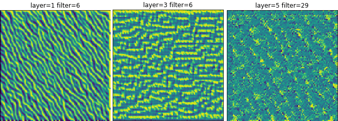
Image 1b: Convolutional layer maps, also looking familiar.

Looking at the conv layer happy maps reveals a couple of things. The first is that the set of HappyMaps produced for both networks are also about the same. The biggest difference in the new set is that there are far fewer of the static or “all on” maps– confirming the suspicion that these types of neurons were not useful. 

Experiment 1-2: Deeper Dense Layers

Our team has often noticed that Google gets incredibly clear pictures of their features, and it makes us wonder how much of an effect our architecture had on it. Of course, there are many experiments that can be run in this regard, but oftentimes it’s best to start with the easiest solutions. In this experiment, we added several more dense layers to deep parts of the network. 

In experiments/experiment1/ex1-2 you will find the notebooks for this experiment. Looking at the training and testing notebooks reveals a similar pattern to experiment0 and ex1-1.

The training accuracy was very high, the testing on the CMU faces testing set was also very high, but the performance on the three amigos was still suboptimal. In fact, the performance on the Ryan dataset was exceptionally bad. Leading us to ask, what does the visualization say?

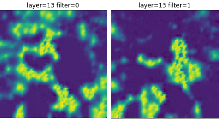
Image 1c: Decision layer maps for experiment 1-2. They look very familiar.

Right off the bat, looking at the decision layer, dense_6 shows that HappyMaps are very similar to what we have already seen. So, this network is not likely to have learned any new tricks — making it almost the same as the others. The convolution and other dense layers are also about the same as previously seen, even though there are quite a bit more of them. This leads us to conclude that these extra dense layers are not doing us any good. 

Experiment 1-3: Wider Dense Layers

Still concerned with how architecture affects learnability, the size of each layer is increased. The notebooks can be found in experiments/experiments1/ex-1-3. The training performance was a little worse, the results on the three amigos was about the same, and more importantly the visualizations are the same. 

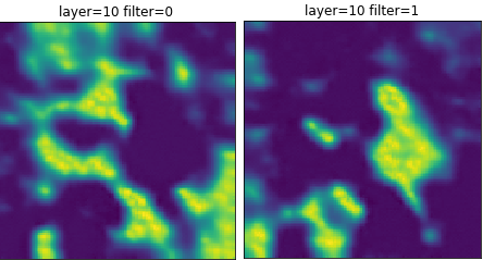
Image 2: Decision layer maps for experiment 1-3. Again, notice the similarities.

This network has learned roughly the same thing as all of the other experiments. The visualizations allow us to clearly state that all of our experiments so far have not significantly altered how the networks perform and how they are going about it. 

Experiment 1-4: The Four Class Problem

This experiment looked to change the problem from just detecting faces left or not, and try to detect if the face is looking left, right, up, or straight. The relevant notebooks are located in experiments/experiments1/ex1-4. The training and the performance on the CMU Faces testing set went well. However, the testing on the three amigos was very poor. The performance on Gilbert and Sarah are roughly the same. The performance on Ryan, however, was a disaster. 

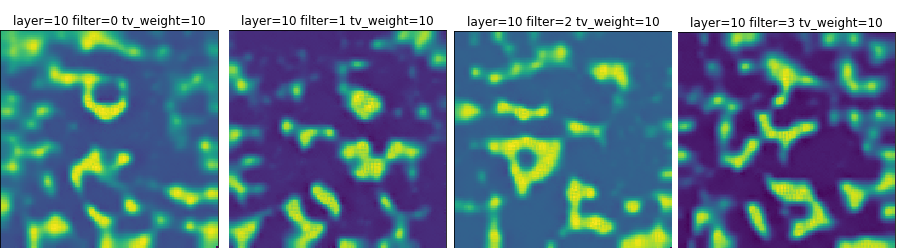
Image 3: Decision layer from 1-4. Filter 0 codes for straight ahead, filter 1 is facing camera left, filter 2 is facing right, and facing 3 is facing up.

Looking at the visualizations, the decision layer is a mess. Frankly, it’s really hard to see what’s been learned. 

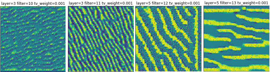
Image 4a: Convolutional layers look similar to others from the past.

The interesting thing to note is that the maps from the convolutional layers are roughly the same as all of the other experiments. This certainly lends credibility to the ideas behind transfer learning. Transfer learning involves taking a network that is already trained and using most of that network in a new task. Since the lower level HappyMaps appear to be the same, perhaps retraining these lower level neurons isn’t needed and focus can shift to the deeper levels. 

Experiment 1-5: Remove the Dense Layers

The purpose of this experience is to see how useful the dense layers are to classification. 

The notebooks for this experiment can be found in experiments/experiments1/ex1-5. Technically, there is one dense layer, the final layer, still present in the model. 

Again, the typical pattern is present: good training results, good testing results, poor results on the three amigos. Even our amiga, Sarah, who is usually respectably classified had poor results.

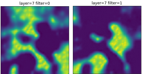
Image 4b: With just a two element dense layer, the familiar maps appear.

Examining the visualizations we see the same pattern. Our decision layer appears to be the same as our other experiments. The convolutional layers are also not terribly different. 

So it would seem that our experiment has confirmed that we just need the one dense layer.  

Experiment 1-6: Remove Softmax

In object classification problems, selecting categorical_crossentropy as the loss function and softmax as the activation function in the decision layer is pretty standard. One of the first observations was that the softmax activation function yields HappyMaps that are complements of each other. Would removing that function produce clearer maps? To test this, the decision layer’s activation function was switched to linear. The loss function was also changed because categorical_crossentropy only works with a softmax activation function. This experiment used the old standby of mean_squared_error. The notebooks can be found in experiments/experiments1/ex1-6. As one might have expected, the training and testing phases were about the same, even with the changes. What’s more exciting are the visualizations. 

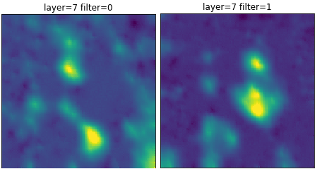
Image 5: Decision layer maps, is this clearer?

First of all, when comparing the decision neurons, they are less complementary. No longer will adding the two maps together yield a perfectly activated map. Looking at the neuron that detects camera left faces, it looks like the activation patterns clearly show a face looking at camera left. Examining the “not left” neuron reveals that it’s more than just “not left”. It’s possible that the activations represent chin positions for looking straight, right, or up. 

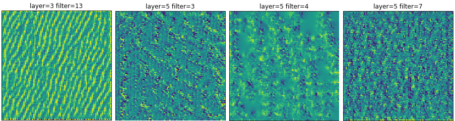
Image 6: Convolutional layer maps. Again, pretty familiar.

Looking at the convolutional layers, they appear to be similar to the other experiments. At this point, conventional wisdom about categorial_crossentropy and softmax seems to hold true. Our previous experiences indicate that these two functions tend to train classification networks faster and more accurately. However, this experiment shows it does produce better visualizations. 

Conclusion

While feature clarity could be better, there’s definitely still value to feature visualization. The first point of appreciation is for the HappyMaps of the output layer. Although the output maps were hard to interpret for the most part, they did help with network optimization efforts. Instead of performing extensive testing to see if network A performed as well as network B, we could simply rely on visualization to see that they had the same HappyMaps. Additionally, the visualizations of the interior layers showed that the layers were larger than necessary. 

Unfortunately, there’s still no insight into how to deal with the biggest problem: the three amigos. Performance on Gilbert, Ryan, and Sarah is still very poor. The visualizations seem to indicate that the facing left neurons are detecting for something that looks like a face looking left. Maybe the network is only looking for that face in a particular location of the image and not generalizing the concept of a left-looking face. Perhaps there’s a tool that can show how the network performs on a given image. Or maybe the key lies in the ability to see what parts of the image the network is attending to, and perhaps this can explain how to fix the network. 

Thanks for keeping up with the Neural Understanding series! We answered a lot of questions along the way, raising a fair number of questions at the same time. In any case, we hope that the insights revealed along the way have provided some food for thought. Who knows, maybe we’ll return in the future to decode more secrets behind neural networks.